Automatic Discretization of a 2D Geometric Obstacle Map

The following is a report I put together for a Technical writing class about some work I did for an "AI for mechanical engineer" class.

Abstract:

The problem of routing pipes and wires around real world obstructions falls under the category of path finding and as such tends to be a computationally complex problem. It can become even more complex than the classical single path problem if many paths need to be found and the choices for them interact, for instance thought space constraints, electronic interference or crosstalk. One approach to reducing the computational load is to reduce the geometric map to an abstract discreet graph and select and evaluate options categorically. This report considers and evaluates techniques for doing this conversion.

Introduction

A number of system layout problems can be broken down into two steps; positioning the major components, and routing the connections between the components. In order for the results from the first step to be automatically evaluated, the second has to be automated. This problem is known as the path finding problem and is known to in general, be of exponential complexity. One way to make this problem more tractable is to convert the obstacle map into a much simpler mathematical graph resulting in a much smaller exponential complexity problem. This will allows more options to be considered and more complex problems to handled.

I have considered two solutions to this problem and, after producing partial solutions to both, determined that one was significantly better and continued that solution to a fully working proof of concept.

The final results only demonstrate a concrete implementation of the concept showing that it is reasonable to compute and that it generates reasonable results. The implementation doesn’t attempt to be more than reasonably efficient.

Discussion

Options Considered

I considered two basic operation principles. The first principle works by finding local maxima for the closest obstacle function. That is to locate positions that can’t be moved away from any nearby obstacles without moving closer to another one. Intuitively this is like inflating a balloon until it fills some region and calling its center a node. These positions were located My implementation used simple hill climbing but partial swarm optimization or simulated annealing might provide better performance.

The second solution worked by locating “pinch points” and treating them as region boundaries. This can be though of as defining rooms by picking what will be counted as a door. The pinch points (doors) were identified by selecting from the lines of closest approach between pairs of obstacles.

General Results

The balloon solution was simpler to implement and, based on preliminary results, tended to generate reasonable results. To generate reliable results over the full map it required many starting locations. This caused it to run very slowly, hampering its usefulness. This might be overcome if some type of dynamic density function could be uses to select more starting locations in smaller passages and fewer in open areas.
The pinch point solution was more complicated to implement but also generate reasonable results and ran many times faster. Based on these results, I chose to only finish implementing this solution.

Restrictions
The final algorithm assumes an input map consisting of non overlapping, convex polygons. The implementation imposes a few more restrictions:

1. The line of closest approach between any two polygons must not share an endpoint with any other for another pair or polygons.
   
2. The map must be bounded by a known set of polygons, in a known order.
   

In practice these might be unnecessary restrictive, for instance some concave polygons might work and some cases of shared line endpoints will work, but the exact conditions where this is allowed are harder to define. Also, improvements in the implementation could allow further relaxation of these requirements.

Methods



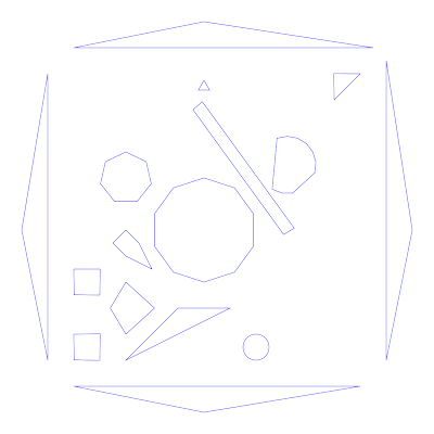
Figure 1: The example input map

I tested the program on an example map was selected to provided a variety of features and scales. These test helped in the development of the program by giving concrete results and by reveling a number of flaws (that were fixed) and limitations (that need to be avoided) during the development process.



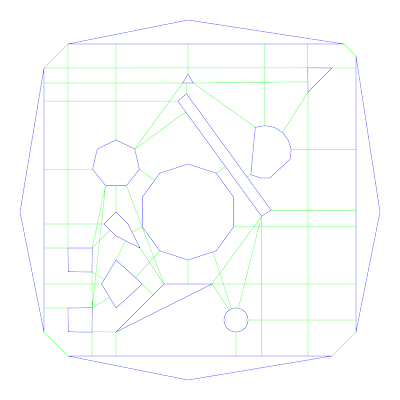
Figure 2: Minimal separation lines

The algorithm operates in several stages. The first stage is feed the initial map and finds the shortest line between each pair of obstacles. Only lines that don’t cross inside of another obstacle are kept.


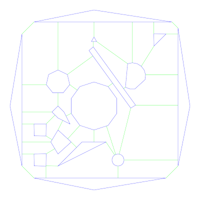
Figure 3: Region boundary selections resulting in a plainer graph.

This set is then filtered to remove crossing lines with a preference for keeping the shortest lines. This results in a plainer graph with the obstacles as nodes and the lines as edges.


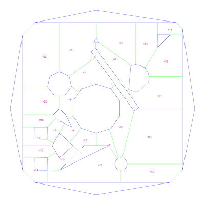
Figure 4: Map with node selection

The interior regions are then identified from this. My implementation does this using a wall following technique. Because all the connecting edges don’t connect to a single point this is somewhat complicated and somewhat of a kluge. To ensure that all interior regions are found, the edges are scanned and each one is traversed exactly once in each directions (this can also be thought of as on both sides) skipping over cases where the edge has been traversed from a previous starting point. This requires either that the exterior edges all be marked from the start as traversed or that the wall following method correctly follow the outside as well.


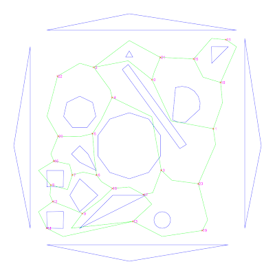
Figure 5: Final graph with nodes and connections

Once the interior sections are identified, the connectivity graph can be found by connecting any two nodes that are bounded from the same link.

Complexity Analysis

1. Finding all links and filtering on overlap with polygons: O(n³) maybe closer to O(n²)
    The number of links is O(n²) and each needs to be checked with each polygon giving the upper case. Better data structures could reduce the cost of the intersection test but not to a constant cost.
   
   
2. Filtering links for overlap: O(n³) maybe closer to O(n²)
    Each of the O(n²) links needs to be checked with each previously accepted link. Given that the result is a plain graph, only O(n) links can be accepted giving the upper bound. Again, with better data structure this might go even lower, but not to a constant.
   
   
3. Region selection: O(n)
    Each of the O(n) links will be traversed twice and each traversal has a cost (for finding the next link) proportional to the O(1) average number of edges per node.
   
4. Connect the regions: O(n)
    This can be done in constant time per link.
   

The worst case, the solution is O(n³), however this might be able to drop to nearer O(n²). Given that this is a precursor to a O(b^d) operation and is cutting back on both b and d, even the worst case result is a clear win for any reasonably sized problem.

Conclusion

My work has show that the basic algorithm of segmenting the map along lines of closets approach is sound. However it also reveals some weaknesses in my implementation. The largest weakness is that the wall following solution is not robust enough to deal with the edges of the map. As this part was not my primary interest I didn’t put much work into it. For a production implementation, it would be worth while to spend some time exploring better options.